ArangoDB and GraphQL

For a while now I’ve been wondering about what might be the minimal set of technologies that allows me to tackle the widest range of projects. The answer I’ve arrived at, for backend development at least, is GraphQL and ArangoDB.

Both of these tools expand my reach as a developer. Projects involving integrations, multiple clients and complicated data that would have been extremely difficult are now within easy reach.

But the minimal set idea is that I can enjoy this expanded range while juggling far fewer technologies than before. Tools that apply in more situations mean fewer things to learn, fewer moving parts and more depth in the learning I do.

While GraphQL and ArangoDB are both interesting technologies individually, it’s in using them together that I’ve been able to realize those benefits; one of those moments where the whole is different from the sum of it’s parts.

Backend Minimalism

My embrace of Javascript has definitely been part of creating that minimal set. A single language for both front and back end development has been a big part of simplifying my tech stack. Both GraphQL and ArangoDB can be used in many languages, but Javascript support is what you might describe as “first among equals” for both projects.

GraphQL can replace, and for me has replaced, server side frameworks like Rails or Django, leaving me with a handful of Javascript functions and more modular, testable code.

GraphQL also replaces ReST, freeing me from thinking about HATEOAS, bike-shedding over the vagaries of ReST, or needing pages and pages of JSON API documentation to save me from bike-shedding over the vagaries of ReST.

ArangoDB has also reduced the number of things I need to need to know. For a start it has removed the “need” for an ORM (no relational database, no need for Object Relational Mapping), which never really delivered on it’s promise to free you from knowing the underlying SQL.

More importantly it’s replaced not just NoSQL databases with a razor-thin set of capabilities like Mongodb (which stores nested documents but can’t do joins) or Neo4j (which does joins but can’t store nested documents), but also general purpose databases like MySQL or Postgres. I have one query language to learn, and one database whose quirks and characteristics I need to know.

It’s also replaced the deeply unpleasant process of relational data modeling with a seamless blend of documents and graphs that make modeling even really ugly connected datasets anticlimactic. As a bonus, in moving the schema outside the database GraphQL lets us enjoy all the benefits of a schema (making sure there is at least some structure I can rely on) and all the benefits of schemalessness (flexibility, ease of change).

Tools that actually reduce the number of things you need to know don’t come along very often. My goal here is to give a sense of what it looks like to use these two technologies together, and hopefully admiring the trees can let us appreciate the forest.

Show me the code

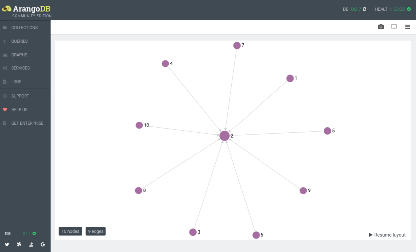
First we need some data to work with. ArangoDB’s administrative interface has some example graphs it can create, so lets use one to explore.

example_graphs

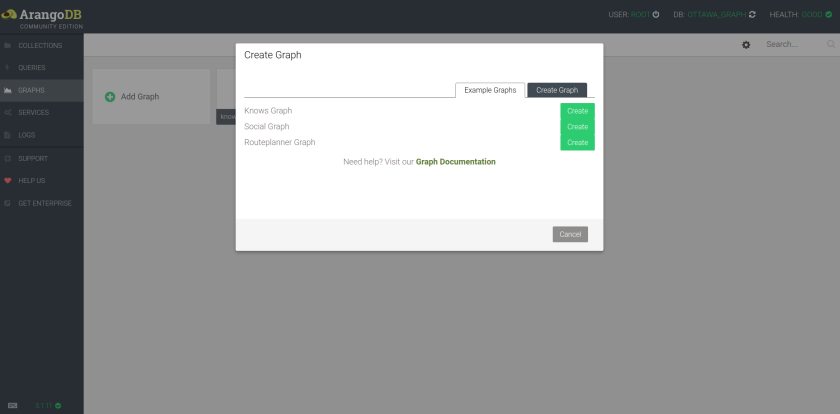
If we select the “knows” graph, we get a simple graph with 5 vertices.

knows_graph

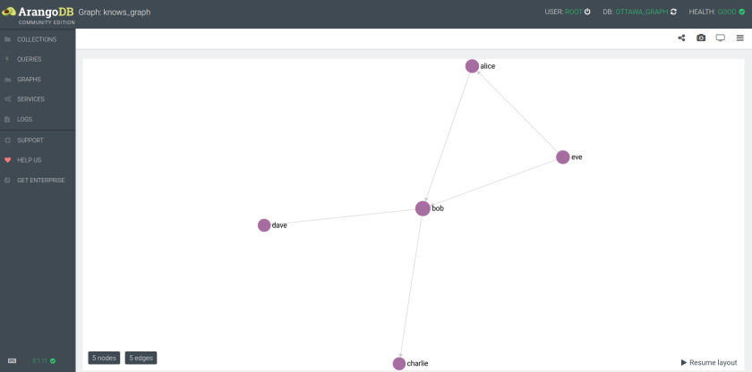
This graph is going to be the foundation for our little exploration.

Next, the only really meaningful information these vertices have is a name attribute. If we are wanting to create a GraphQL type that represents one of these objects it would look like this:

  let Person = new GraphQLObjectType({
    name: 'Person',
    fields: () => ({
      name: {
        type: GraphQLString
      }
    })
  })

Now that we have a type that describes what a Person object looks like we can use it in a schema. This schema has a field called person which has two attributes: type, and resolve.

let schema = new GraphQLSchema({
    query: new GraphQLObjectType({
      name: 'Query',
      fields: () => ({
        person: {
          type: Person,
          resolve: () => {
            return {name: 'Mike'}
          },
        }
      })
    })
  })

The resolve is a function that will be run whenever graphql is asked to produce a person object. type is a type that describes the object that the resolve function returns, which in this this case is our Person type.

To see if this all works we can write a test using Jest.

import {
  graphql,
  GraphQLSchema,
  GraphQLObjectType,
  GraphQLString,
  GraphQLList,
  GraphQLNonNull
} from 'graphql'

describe('returning a hardcoded object that matches a type', () => {

  let Person = new GraphQLObjectType({
    name: 'Person',
    fields: () => ({
      name: {
        type: GraphQLString
      }
    })
  })

  let schema = new GraphQLSchema({
    query: new GraphQLObjectType({
      name: 'Query',
      fields: () => ({
        person: {
          type: Person,
          resolve: () => {
            return {name: 'Mike'}
          },
        }
      })
    })
  })

  it('lets you ask for a person', async () => {

    let query = `
      query {
        person {
          name
        }
      }
    `;

    let { data } = await graphql(schema, query)
    expect(data.person).toEqual({name: 'Mike'})
  })

})

This test passes which tells us that we got everything wired together properly, and the foundation laid to talk to ArangoDB.

First we’ll use arangojs and create a db instance and then a function that allows us to get a person using their name.

//src/database.js
import arangojs, { aql } from 'arangojs'

export const db = arangojs({
  url: `http://${process.env.ARANGODB_USER}:${process.env.ARANGODB_PASSWORD}@127.0.0.1:8529`,
  databaseName: 'knows'
})

export async function getPersonByName (name) {
  let query = aql`
      FOR person IN persons
        FILTER person.name == ${ name }
          LIMIT 1
          RETURN person
    `
  let results = await db.query(query)
  return results.next()
}

Now lets use that function with our schema to retrieve real data from ArangoDB.

import {
  graphql,
  GraphQLSchema,
  GraphQLObjectType,
  GraphQLString,
  GraphQLList,
  GraphQLNonNull
} from 'graphql'
import {
  db,
  getPersonByName
} from '../src/database'

describe('queries', () => {

  it('lets you ask for a person from the database', async () => {

    let Person = new GraphQLObjectType({
      name: 'Person',
      fields: () => ({
        name: {
          type: GraphQLString
        }
      })
    })

    let schema = new GraphQLSchema({
      query: new GraphQLObjectType({
        name: 'Query',
        fields: () => ({
          person: {
            args: { //person now accepts args
              name: { // the arg is called "name"
                type: new GraphQLNonNull(GraphQLString) // name is a string & manadatory
              }
            },
            type: Person,
            resolve: (root, args) => {
              return getPersonByName(args.name)
            },
          }
        })
      })
    })

    let query = `
        query {
          person(name "Eve") {
            name
          }
        }
      `

    let { data } = await graphql(schema, query)
    expect(data.person).toEqual({name: 'Eve'})
  })
})

Here we have modified our schema to accept a name argument when asking for a person. We access the name via the args object and pass it to our database function to go get the matching person from Arango.

Let’s add a new database function to get the friends of a user given their id.
What’s worth pointing out here is that we are using ArangoDB’s AQL traversal syntax. It allows us to do a graph traversal across outbound edges get the vertex on the other end of the edge.

export async function getFriends (id) {
  let query = aql`
      FOR vertex IN OUTBOUND ${id} knows
        RETURN vertex
    `
  let results = await db.query(query)
  return results.all()
}

Now that we have that function, instead of adding it to the schema, we add a field to the Person type. In the resolve for our new friends field we are going to use the root argument to get the id of the current person object and then use our getFriends function to do the traveral to retrieve the persons friends.

    let Person = new GraphQLObjectType({
      name: 'Person',
      fields: () => ({
        name: {
          type: GraphQLString
        },
        friends: {
          type: new GraphQLList(Person),
          resolve(root) {
            return getFriends(root._id)
          }
        }
      })
    })

What’s interesting is that because of GraphQL’s recursive nature, this change lets us query for friends:

        query {
          person(name: "Eve") {
            name
            friends {
              name
            }
          }
        }

and also ask for friends of friends (and so on) like this:

        query {
          person(name: "Eve") {
            name
            friends {
              name
              friends {
                name
              }
            }
          }
        }

We can show that with a test.

import {
  graphql,
  GraphQLSchema,
  GraphQLObjectType,
  GraphQLString,
  GraphQLList,
  GraphQLNonNull
} from 'graphql'
import {
  db,
  getPersonByName,
  getFriends
} from '../src/database'

describe('queries', () => {

  it('returns friends of friends', async () => {

    let Person = new GraphQLObjectType({
      name: 'Person',
      fields: () => ({
        name: {
          type: GraphQLString
        },
        friends: {
          type: new GraphQLList(Person),
          resolve(root) {
            return getFriends(root._id)
          }
        }
      })
    })

    let schema = new GraphQLSchema({
      query: new GraphQLObjectType({
        name: 'Query',
        fields: () => ({
          person: {
            args: {
              name: {
                type: new GraphQLNonNull(GraphQLString)
              }
            },
            type: Person,
            resolve: (root, args) => {
              return getPersonByName(args.name)
            },
          }
        })
      })
    })

    let query = `
        query {
          person(name: "Eve") {
            name
            friends {
              name
              friends {
                name
              }
            }
          }
        }
      `

    let result = await graphql(schema, query)
    let { friends } = result.data.person
    let foaf = [].concat(...friends.map(friend => friend.friends))
    expect([{name: 'Charlie'},{name: 'Dave'},{name: 'Bob'}]).toEqual(expect.arrayContaining(foaf))
  })

})

This test has running a query three levels deep and walking the entire graph. Because we can ask for any combination of any of the things our types defined, we have a whole lot of flexibility with very little code. The code that’s there is just a few simple functions, modular and easy to test.

But what did we trade away to get all that? If we look at the queries that get sent to Arango with tcpdump we can see how that sausage was made.

// getPersonByName('Eve') from the person resolver in our schema 
{"query":"FOR person IN persons
  FILTER person.name == @value0
  LIMIT 1 RETURN person","bindVars":{"value0":"Eve"}}
// getFriends('persons/eve') in Person type -> returns Bob & Alice.
{"query":"FOR vertex IN OUTBOUND @value0 knows
  RETURN vertex","bindVars":{"value0":"persons/eve"}}
// now a new request for each friend:
// getFriends('persons/bob')
{"query":"FOR vertex IN OUTBOUND @value0 knows
  RETURN vertex","bindVars":{"value0":"persons/bob"}}
// getFriends('persons/alice')
{"query":"FOR vertex IN OUTBOUND @value0 knows
  RETURN vertex","bindVars":{"value0":"persons/alice"}}

What we have here is our own version of the famous N+1 problem. If we were to add more people to this graph things would get out of hand quickly.

Facebook, which has been using GraphQL in production for years, is probably even less excited about the prospect of N+1 queries battering their database than we are. So what are they doing to solve this?

Using Dataloader

Dataloader is a small library released by Facebook that solves the N+1 problem by cleverly leveraging the way promises work. To use it, we need to give it a batch loading function and then replace our calls to the database with calls call Dataloader’s load method in all our resolves.

What, you might ask, is a batch loading function? The dataloader documentation offers that “A batch loading function accepts an Array of keys, and returns a Promise which resolves to an Array of values.”

We can write one of those.

async function getFriendsByIDs (ids) {
  let query = aql`
    FOR id IN ${ ids }
      let friends = (
        FOR vertex IN OUTBOUND id knows
          RETURN vertex
      )
      RETURN friends
  `
  let response = await db.query(query)
  return response.all()
}

We can then use that in a new test.

import {
  graphql
} from 'graphql'
import DataLoader from 'dataloader'
import {
  db,
  getFriendsByIDs
} from '../src/database'
import schema from '../src/schema'

describe('Using dataloader', () => {

  it('returns friends of friends', async () => {

    let Person = new GraphQLObjectType({
      name: 'Person',
      fields: () => ({
        name: {
          type: GraphQLString
        },
        friends: {
          type: new GraphQLList(Person),
          resolve(root, args, context) {
            return context.FriendsLoader.load(root._id)
          }
        }
      })
    })

    let query = `
        query {
          person(name: "Eve") {
            name
            friends {
              name
              friends {
                name
              }
            }
          }
        }
      `
    const FriendsLoader = new DataLoader(getFriendsByIDs)
    let result = await graphql(schema, query, {}, { FriendsLoader })
    let { person } = result.data
    expect(person.name).toEqual('Eve')
    expect(person.friends.length).toEqual(2)
    let names = person.friends.map(friend => friend.name)
    expect(names).toContain('Alice', 'Bob')
  })

})

The key section of the above test is this:

    const FriendsLoader = new DataLoader(getFriendsByIDs)
    //                         schema, query, root, context
    let result = await graphql(schema, query, {}, { FriendsLoader })

The context object is passed as the fourth parameter to the graphql function which is then available as the third parameter in every resolve function. With our FriendsLoader attached to the context object, you can see us accessing it in the resolve function on the Person type.

Let’s see what effect that batch loading has on our queries.

// getPersonByName('Eve') from the person resolver in our schema 
{"query":"FOR person IN persons
  FILTER person.name == @value0
  LIMIT 1 RETURN person","bindVars":{"value0":"Eve"}}
// getFriendsByIDs(["persons/eve"]) -> returns Bob & Alice.
{"query":"FOR id IN @value0
   let friends = (
    FOR vertex IN  OUTBOUND id knows
      RETURN vertex
    )
  RETURN friends","bindVars":{"value0":["persons/eve"]}}
// getFriendsByIDs(["persons/alice","persons/bob"])
{"query":"FOR id IN @value0
   let friends = (
    FOR vertex IN  OUTBOUND id knows
      RETURN vertex
    )
  RETURN friends","bindVars":{"value0":["persons/alice","persons/bob"]}}

Now for a three level query (Eve, her friends, their friends) we are down to just 1 query per level and the N+1 problem is no longer a problem.

When it’s time to serve your data to the world, express-graphql supplies a middleware that we can pass our schema and loaders to like this:

import express from 'express'
import graphqlHTTP from 'express-graphql'
import schema from './schema'
import DataLoader from 'dataloader'
import { getFriendsByIDs } from '../src/database'

const FriendsLoader = new DataLoader(getFriendsByIDs)
const app = express()
app.use('/graphql', graphqlHTTP({ schema, context: { FriendsLoader }}))
app.listen(3000)
// http://localhost:3000/graphql is up and running!

What we just did

With just those few code examples we’ve built a backend system that provides a query-able API for clients backed by a graph database. Growing it would look like adding a few more functions and a few more types. The code stays modular and testable. Dataloader has ensured that we didn’t even pay a performance penalty for that.

A perfect combination

While geeking out on the technology is fun, it loses sight of what I think is the larger point: The design of both GraphQL and ArangoDB allow you to combine and recombine some really simple primitives to tackle anything you can think of.

With ArangoDB, it’s all just documents, whether you use them like that or treat them as key/value or a graph is up to you. While this approach is marketed as “multi-model” database, the term is unfortunate since it makes the database sound like it’s trying to do lots of things instead of leveraging some fundamental similarity between these types of data. That similarity becomes the “primitive” that makes all this flexibility possible.

For GraphQL, my application is just a bunch of functions in an Abstract Syntax Tree which get combined and recombined by client queries. The parser and execution engine take care of what gets called when.

In each case what I need to understand is simple, the behaviour I can produce is complex.

I’m still honing my minimal set for front end development, but for backend development this is now how I build. These days I’m refocusing my learning to go narrow and deep and it feels good. Infinite width never felt sustainable. It’s not apparent at first, but once that burden is lifted off your shoulders you will realize how heavy it was.

Dealing with supernodes in ArangoDB

About a year ago I wrote about data modeling in ArangoDB. The main take away is to avoid the temptation to make unnecessary vertices (and all the attendant edges), since the traversing high degree vertices (a vertex with lots of edges pointing at it) is an expensive process.

Graphs are cool and it’s easy to forget that ArangoDB is a great document store. Treating is as such means “Embedding“, to borrow a term from MongoDB,  which lets you keep your traversals fast.

But while good data modeling can prevent you from creating some high-degree vertices, you will run into them eventually, and ArangoDB’s new “vertex-centric” indexes is a feature that is there for exactly those moments.

First we can try and get a sense of the impact these high-degree vertices have on a traversal. To do that I wrote a script that would generate a star graph starting with three “seed” vertices, a start, middle, and end.

The goal was to walk across the middle vertex to get from start to end while changing the number of vertices connected to the middle.

// the seed vertices
let seedVertices = [
  {name: 'start', _key: '1', type: "seed"},
  {name: 'middle', _key: '2', type: "seed"},
  {name: 'end', _key: '3', type: "seed"}
]

With just 10 vertices, this is nowhere near deserving the name “supernode”, but it’s pretty clear why these things are called star-graphs.

star_graph
A baby “super node”.

Next we crank up the number of vertices so we can see the effect on traversal time.

star_graph_traversal

By the time we get to a vertex surrounded by 100,000 to 1,000,000 other vertices we are starting to get into full-blown supernode territory. You can see that by the time we get to sorting through a million incident edges ArangoDB is up to 4.3 seconds to traverse across that middle vertex.

A “vertex-centric” index is one that include either _to or _from plus some other edge attribute. In this case I’ve added a type attribute which I’ll combine with _to to make my index. (Note that if I was allowing “any” as a direction I would need a second index that combines type and _from)

creating_a_hash_index

ArangoDB calculates the path and offers it to you as you do a traversal. You can access the path by declaring a variable to receive it. In the query below p contains the path. If we use the ALL array comparison operator on p.edges to say that all the edges in the path should have type of “seed”, that should be enough to get Arango to use are new index.

    FOR v,e,p IN 1..2 ANY 'vertices/1' edges
      FILTER p.edges[*].type ALL == 'seed' &&  v.name == 'end'
        RETURN v

The selectivity score shown by explain doesn’t leave you very hopeful that Arango will use the index…

Indexes used:
 By   Type   Collection   Unique   Sparse   Selectivity   Fields               Ranges
  2   hash   edges        false    false         0.00 %   [ `type`, `_to` ]    base INBOUND
  2   edge   edges        false    false        50.00 %   [ `_from`, `_to` ]   base OUTBOUND

but having our query execute in 0.2 milliseconds instead of 4.3 seconds is a pretty good indication it’s working.

arango_query_explained

Back to modeling

For me, this little experiment has underscored the importance of good data modeling. You don’t have to worry about the number of edges if you don’t create a vertex in the first place. If you are conservative about what you are willing to make a vertex, and make good use of indexes you can see that ArangoDB is going to be able to gracefully handle some pretty hefty data.

With vertex-centric indexes, and other features like the new Smartgraphs, ArangoDB has gone from being a great document database with a trick up it’s sleeve (Joins!) to being a really solid graph database and there are new features landing regularly. I’m curious to see where they go next.

Graph traversals in ArangoDB

ArangoDB’s AQL query language was created to offer a unified interface for working with key/value, document and graph data. While AQL has been easy to work with and learn, it wasn’t until the addition of AQL traversals in ArangoDB 2.8 that it really felt like it has achieved it’s goal.

Adding keywords GRAPH, OUTBOUND, INBOUND and ANY suddenly made iteration using a FOR loop the central idea in the language. This one construct can now be used to iterate over everything; collections, graphs or documents:

//FOR loops for everything
FOR person IN persons //collections
  FOR friend IN OUTBOUND person GRAPH "knows_graph" //graphs
    FOR value in VALUES(friend, true) //documents
    RETURN DISTINCT value

AQL has always felt more like programming than SQL ever did, but the central role of the FOR loop gives a clarity and simplicity that makes AQL very nice to work with. While this is a great addition to the language, it does however, mean that there are now 4 different ways to traverse a graph in AQL and a few things are worth pointing out about the differences between them.

AQL Traversals

There are two variations of the AQL traversal syntax; the named graph and the anonymous graph. The named graph version uses the GRAPH keyword and a string indicating the name of an existing graph. With the anonymous syntax you can simply supply the edge collections

//Passing the name of a named graph
FOR vertex IN OUTBOUND "persons/eve" GRAPH "knows_graph"
//Pass an edge collection to use an anonymous graph
FOR vertex IN OUTBOUND "persons/eve" knows

Both of these will return the same result. The traversal of the named graph uses the vertex and edge collections specified in the graph definition, while the anonymous graph uses the vertex collection names from the _to/_from attributes of each edge to determine the vertex collections.

If you want access to the edge or the entire path all you need to do is ask:

FOR vertex IN OUTBOUND "persons/eve" knows
FOR vertex, edge IN OUTBOUND "persons/eve" knows
FOR vertex, edge, path IN OUTBOUND "persons/eve" knows

The vertex, edge and path variables can be combined and filtered on to do some complex stuff. The Arango docs show a great example:

FOR v, e, p IN 1..5 OUTBOUND 'circles/A' GRAPH 'traversalGraph'
  FILTER p.edges[0].theTruth == true
  AND p.edges[1].theFalse == false
  FILTER p.vertices[1]._key == "G"
  RETURN p

Notes

Arango can end up doing a lot of work to fill in those FOR v, e, p IN variables. ArangoDB is really fast, so to show the effect these variables can have, I created the most inefficient query I could think of; a directionless traversal across a high degree vertex with no indexes.

The basic setup looked like this except with 10000 vertices instead of 10. The test was getting from start across the middle vertex to end.

Screenshot from 2016-04-05 10-07-04

What you can see is that adding those variables comes at a cost, so only declare ones you actually need.

effects_of_traversal_variables
Traversing a supernode with 10000 incident edges with various traversal methods. N=5. No indexes used.

GRAPH_* functions and TRAVERSAL

ArangoDB also has a series of “Named Operations” that feature among
them a few that also do traversals. There is also a super old-school TRAVERSAL function hiding in the “Other” section. What’s interesting is how different their performance can be while still returning the same results.

I tested all of the traversal functions on the same supernode described above. These are the queries:

//AQL traversal
FOR v IN 2 ANY "vertices/1" edges
  FILTER v.name == "end"
    RETURN v

//GRAPH_NEIGHBORS
RETURN GRAPH_NEIGHBORS("db_10000", {_id: "vertices/1"}, {direction: "any", maxDepth:2, includeData: true, neighborExamples: [{name: "end"}]})

//GRAPH_TRAVERSAL
RETURN GRAPH_TRAVERSAL("db_10000", {_id:"vertices/1"}, "any", {maxDepth:2, includeData: true, filterVertices: [{name: "end"}], vertexFilterMethod: ["exclude"]})

//TRAVERSAL
RETURN TRAVERSAL(vertices, edges, {_id: "vertices/1"}, "any", {maxDepth:2, includeData: true, filterVertices: [{name: "end"}], vertexFilterMethod: ["exclude"]})

All of these returned the same vertex, just with varying levels of nesting within various arrays. Removing the nesting did not make a signficant difference in the execution time.

traversal_comparison
Traversing a supernode with 10000 incident edges with various traversal methods. N=5.

Notes

While TRAVERSAL and GRAPH_TRAVERSAL were not stellar performers here, the both have a lot to offer in terms of customizability. For ordering, depthfirst searches and custom expanders and visitors, this is the place to look. As you explore the options, I’m sure these get much faster.

Slightly less obvious but still worth pointing out that where AQL traversals require an id (“vertices/1000” or a document with and _id attribute), GRAPH_* functions just accept an example like {foo: “bar”} (I’ve passed in {_id: “vertices/1”} as the example just to keep things comparable). Being able to find things, without needing to know a specific id, or what collection to look in is very useful. It lets you abstract away document level concerns like collections and operate on a higher “graph” level so you can avoid hardcoding collections into your queries.

What it all means

The difference between these, at least superficially, similar traversals are pretty surprising. While some where faster than others, none of the options for tightening the scope of the traversal were used (edge restrictions, indexes, directionality). That tells you there is likely a lot of headroom for performance gains for all of the different methods.

The conceptual clarity that AQL traversals bring to the language as a whole is really nice, but it’s clear there is some optimization work to be done before I go and rewrite all my queries.

Where I have used the new AQL traversal syntax, I’m also going to have to check to make sure there are no unused v,e,p variables hiding in my queries. Where you need to use them, it looks like restricting yourself to v,e is the way to go. Generating those full paths is costly. If you use them, make sure it’s worth it.

Slowing Arango down is surprisingly instructive, but with 3.0 bringing the switch to Velocypack for JSON serialization, new indexes, and more, it looks like it’s going to get harder to do. :)


A quick tour of Arangojs

I’ve been using ArangoDB for a while now, but for most of that time I’ve been using it from Ruby. I’ve dabbled with the Guacamole library and even took a crack at writing my own, but switching to Javascript has led me to get to know Arangojs.

Given that Arangojs is talking to ArangoDB via its HTTP API, basically everything you do is asynchronous. There are a few ways of dealing with async code in Javascript, and Arangojs has been written to support basically all of them.

Arangojs’s flexibility and my inexperience with the new Javascript syntax combined to give me bit of an awkward start, so with a little learning under my belt I thought I would write up some examples that would have saved me some time.

My most common use case is running an AQL query, so lets use that as an example. First up, I’ve been saving my config in a separate file:

// arango_config.js
//Using auth your url would look like:
// "http://uname:passwd@127.0.0.1:8529"
module.exports = {
  "production" : {
    "databaseName": process.env.PROD_DB_NAME,
    "url": process.env.PROD_DB_HOST,
  },
  "development" : {
    "databaseName": process.env.DEVELOPMENT_DB_NAME,
    "url": process.env.DEVELOPMENT_URL
  },
  "test" : {
    "databaseName": "test",
    "url": "http://127.0.0.1:8529",
  },
}

With that I can connect to one of my existing databases like so:

var config = require('../arangodb_config')[process.env.NODE_ENV]
var db = require('arangojs')(config)

This keeps my test database nicely separated from everything else and all my db credentials in the environment and out of my project code.

Assuming that our test db has a collection called “documents” containing a single document, we can use Arangojs to go get it:

db.query('FOR doc IN documents RETURN doc', function(err, cursor) {
  cursor.all(function(err, result) {
    console.log(result)
  })
})

Which returns:

[ { foo: 'bar',
    _id: 'documents/206191358605',
    _rev: '206192931469',
    _key: '206191358605' } ]

While this is perfectly valid Javascript, its pretty old-school at this point since ECMAScript 2015 is now standard in both Node.js and any browser worth having. This means we can get rid of the “function” keyword and replace it with the “fat arrow” syntax and get the same result:

db.query('FOR doc IN documents RETURN doc', (err, cursor) => {
  cursor.all((err, result) => {
    console.log(result)
  })
})

So far so good but the callback style (and the callback-hell it brings) is definitely an anti-pattern. The widely cited antidote to this is promises:

db.query('FOR doc IN documents RETURN doc')
  .then((cursor) => { return cursor.all() })
  .then((doc) => { console.log(doc) });

While this code is functionally equivalent, it operates by chaining promises together. While it’s an improvement over callback-hell, after writing a bunch of this type of code, I ended up feeling like I had replaced callback hell with promise hell.

what-fresh-hell-is-this

The path back to sanity lies in ECMAScript 2016 aka ES7 and the new async/await keywords. Inside a function marked as async, you have access to an await keyword which allows you to write code that looks synchronous but does not block the event loop.

Using the babel transpiler lets us use the new ES7 syntax right now by compiling it all down to ES5/6 equivalents. Installing with npm install -g babel and running your project with babel-node is all that you need to be able to write this:

async () => {
    let cursor = await db.query('FOR doc IN documents RETURN doc')
    let result = await cursor.all()
    console.log(result)
}()

Once again we get the same result but without all the extra cruft that we would normally have to write.

One thing that is notably absent in these examples is the use of bound variables in our queries to avoid SQL injection (technically parameter injection since this is NoSQL).

So what does that look like?

async () => {
    let bindvars = {foo: "bar"}
    let cursor = await db.query('FOR doc IN documents FILTER doc.foo == @foo RETURN doc', bindvars)
    let result = await cursor.all()
    console.log(result)
}()

But Arangojs lets you go further, giving you a nice aqlQuery function based on ES6 template strings:

async () => {
    let foo = "bar"
    let aql = aqlQuery`
      FOR doc IN documents
        FILTER doc.foo == ${foo}
          RETURN doc
    `
    let cursor = await db.query(aql)
    let result = await cursor.all()
    console.log(result)
}()

Its pretty astounding how far that simple example has come. It’s hard to believe that it’s even the same language.
With Javascript (the language and the community) clearly in transition, Arangojs (and likely every other JS library) is compelled to support both the callback style and promises. It’s a bit surprising to see how much leeway that gives me to write some pretty sub-optimal code.

With all the above in mind, suddenly Arangojs’s async heavy API no longer feels intimidating.

The documentation for Arangojs is simple (just a long readme file) but comprehensive and there is lots more it can do. Hopefully this little exploration will help people get started with Arangojs a little more smoothly than I did.

Extracting test data from ArangoDB’s admin interface

Test Driven Development is an important part of my development process and
ArangoDB’s speed, schema-less nature and truncate command make testing really nice.

Testing has ended up being especially important to me when it comes to AQL (Arango Query Language) queries. Just the same way that its easy to write a regular expression that matches more than you expect, constraining the traversal algorithm so you get what you want (and only that) can be tricky.

AQL queries that traverse a graph are often (maybe always?) sensitive to the structure of the graph. The direction of the edges (inbound/outbound) or the number of edges to cross (maxDepth) are often used to constrain a traversal. Both of these are examples of how details of your graphs structure get built into your AQL queries. When the structure isn’t what you think, you can end up with some pretty surprising results coming back from your queries.

All of that underscores the need to test against data that you know has a specific structure. A few times now I have found myself with bunch of existing graph data, and wondering how to pick out a selected subgraph to test my AQL queries against.

ArangoDB’s web interface gets me tantalizingly close, letting me filter down to a single starting node and clicking with the spot tool to reveal its neighbors.

Filtering for a specific vertex in the graph.

In a few clicks I can get exactly the vertices and edges that I need to test my queries, and because I have seen it, I know the structure is correct, and has only what I need. All that is missing is a way to save what I see.

Since this seems to keep coming up for me, I’ve solved this for myself with a little hackery that I’ve turned to several times now. The first step is turning on Firefox’s dump function by entering about:config in the URL bar and searching the settings for “dump”.

Firefox can dump to the terminal with browser.dom.window.dump.enabled

The dump function allows you to write to the terminal from javascript. Once that is set to true, launching Firefox from the terminal, and typing dump("foo") in the Javascript console should print “foo” in the controlling terminal.

test_data

Next, since the graph viewer uses D3 to for its visualization, we can dig into the DOM and print out the bits we need using dump. Pasting the following into the Javascript console will print out the edges:

var edges = document.querySelector('#graphViewerSVG').childNodes[0].childNodes[0].children; for(var i = 0; i < edges.length; i++) { dump("\r\n" + JSON.stringify(edges[i].__data__._data) + "\r\n"); }

And then this will print out the vertices:

var vertices = document.querySelector('#graphViewerSVG').childNodes[0].childNodes[1].children; for(var i = 0; i < vertices.length; i++) { dump("\r\n" + JSON.stringify(vertices[i].__data__._data) + "\r\n"); }

With the vertices and edges now printed to the terminal, a little copy/paste action and you can import the data into your test database before running your tests with arangojs’s import function.

myCollection.import([
  {foo: "bar"},
  {fizz: "buzz"}
])

Alternately you can upload JSON files into the collection via the web interface as well.

Importing JSON into a collection.

While this process has no claim on elegance, its been very useful for testing my AQL queries and saved me a lot of hassle.

Data modeling with ArangoDB

Since 2009 there has been a “Cambrian Explosion” of NoSQL databases, but information on data modeling with these new data stores feels hard to come by.
My weapon of choice for over a year now has been ArangoDB. While ArangoDB is pretty conscientious about having good documentation, there has been something missing for me: criteria for making modeling decisions.

Like most (all?) graph databases, ArangoDB allows you to model your data with a property graph. The building blocks of a property graph are attributes, vertices and edges. What makes data modelling with ArangoDB (and any other graph database) difficult is deciding between them.

To start with we need a little terminology. Since a blog is a well known thing, we can use a post with some comments and some tags as our test data to illustrate the idea.

Sparse vs Compact

Modeling our blog post with as a “sparse” graph might look something like this:

sparse

At first glance it looks satisfyingly graphy: in the centre we see a green “Data Modeling” vertex which has a edge going to another vertex “post”, indicating that “Data Modeling” is a post. Commenters, tags and comments all have connections to a vertex representing their type as well.

Looking at the data you can see we are storing lots of edges and most vertices contain only a single attribute (apart from the internal attributes ArangoDB creates: _id, _key, _rev).

//vertices
{"_id":"vertices/26590247555","_key":"26590247555","_rev":"26590247555","title":"That's great honey","text":"Love you!"},
{"_id":"vertices/26590378627","_key":"26590378627","_rev":"26590378627","type":"comment"},
{"_id":"vertices/26590509699","_key":"26590509699","_rev":"26590509699","name":"Spammy McSpamerson","email":"spammer@fakeguccihandbags.com"},
{"_id":"vertices/26590640771","_key":"26590640771","_rev":"26590640771","title":"Brilliant","text":"Gucci handbags..."},
{"_id":"vertices/26590771843","_key":"26590771843","_rev":"26590771843","name":"arangodb"},
{"_id":"vertices/26590902915","_key":"26590902915","_rev":"26590902915","name":"modeling"},
{"_id":"vertices/26591033987","_key":"26591033987","_rev":"26591033987","name":"nosql"},
{"_id":"vertices/26591165059","_key":"26591165059","_rev":"26591165059","type":"tag"}]
 
//edges
[{"_id":"edges/26604010115","_key":"26604010115","_rev":"26604010115","_from":"vertices/26589723267","_to":"vertices/26589395587"},
{"_id":"edges/26607352451","_key":"26607352451","_rev":"26607352451","_from":"vertices/26589723267","_to":"vertices/26589854339"},
{"_id":"edges/26608204419","_key":"26608204419","_rev":"26608204419","_from":"vertices/26590640771","_to":"vertices/26590378627"},
{"_id":"edges/26609842819","_key":"26609842819","_rev":"26609842819","_from":"vertices/26590247555","_to":"vertices/26590378627"},
{"_id":"edges/26610694787","_key":"26610694787","_rev":"26610694787","_from":"vertices/26589985411","_to":"vertices/26590247555"},
{"_id":"edges/26611546755","_key":"26611546755","_rev":"26611546755","_from":"vertices/26589395587","_to":"vertices/26590247555"},
{"_id":"edges/26615020163","_key":"26615020163","_rev":"26615020163","_from":"vertices/26589985411","_to":"vertices/26590116483"},
{"_id":"edges/26618821251","_key":"26618821251","_rev":"26618821251","_from":"vertices/26590771843","_to":"vertices/26591165059"},
{"_id":"edges/26622622339","_key":"26622622339","_rev":"26622622339","_from":"vertices/26589395587","_to":"vertices/26589592195"},
{"_id":"edges/26625833603","_key":"26625833603","_rev":"26625833603","_from":"vertices/26590509699","_to":"vertices/26590640771"},
{"_id":"edges/26642741891","_key":"26642741891","_rev":"26642741891","_from":"vertices/26589395587","_to":"vertices/26590902915"},
{"_id":"edges/26645101187","_key":"26645101187","_rev":"26645101187","_from":"vertices/26589395587","_to":"vertices/26590771843"},
{"_id":"edges/26649885315","_key":"26649885315","_rev":"26649885315","_from":"vertices/26589395587","_to":"vertices/26591033987"},
{"_id":"edges/26651064963","_key":"26651064963","_rev":"26651064963","_from":"vertices/26590902915","_to":"vertices/26591165059"},
{"_id":"edges/26651785859","_key":"26651785859","_rev":"26651785859","_from":"vertices/26591033987","_to":"vertices/26591165059"},
{"_id":"edges/26652965507","_key":"26652965507","_rev":"26652965507","_from":"vertices/26590509699","_to":"vertices/26590116483"},
{"_id":"edges/26670267011","_key":"26670267011","_rev":"26670267011","_from":"vertices/26589395587","_to":"vertices/26590640771"}]

A “compact” graph on the other hand might look something like this:

{
  title: "Data modelling",
  text: "lorum ipsum...",
  author: "Mike Williamson",
  date: "2015-11-19",
  comments: [
    {
      author:"Mike's Mum",
      email:"mikes_mum@allthemums.com",
      text: "That's great honey",
    },
    {
      "author": "spammer@fakeguccihandbags.com",
      "title": "Brilliant",
      "text": "Gucci handbags...",
    }
  ],
  tags:["mongodb","modeling","nosql"]
}

Here we have taken exactly the same data and collapsed it together into a single document. While its a bit of a stretch to even classify this as a graph, ArangoDB’s multi-model nature largely erases the boundary between a document and a graph with a single vertex.

The two extremes above give us some tools for talking about our graph. Its the same data either way, but clearly different choices are being made. In the sparse graph, every vertex you see could have been an attribute, but was consciously moved into a vertex of its own. The compact graph is what comes out of repeated choosing to add new data as an attribute rather than a vertex.

When modeling real data your decisions don’t always fall one one side or the other. So what criteria should we be using to make those decisions?

Compact by default

As a baseline you should favor a compact graph. Generally data that is displayed together should be combined into a single document.

Defaulting to compact will mean fewer edges will exist in the graph as a whole. Since each traversal across a graph will have to find, evaluate and then traverse the edges for each vertex it encounters, keeping the number of edges to a strict minimum will ensure traversals stay fast as your graph grows.
Compact graphs will also mean fewer queries and traversals to get the information you need. When in doubt, embed. Resist the temptation to add vertices just because it’s a graph database, and keep it compact.

But not everything belongs together. Any attribute that contains a complex data structure (like the “comments” array or the “tags” array) deserves a little scrutiny as it might make sense as a vertex (or vertices) of its own.

Looking at our compact graph above, the array of comments, the array of tags, and maybe even the author might be better off as vertices rather than leaving them as attributes. How do we decide?

  • Will it be accessed on it’s own? (ie: showing comments without the post)
  • Will you be running a graph measurement (like GRAPH_BETWEENNESS) on it?
  • Will it be edited on it’s own?
  • Does/could the attribute have relationships of it’s own? (assuming you care)
  • Would/should this attribute exist without it’s parent vertex?

Removing duplicate data can also be a reason to make something a vertex, but with the cost of storage ridiculously low (and dropping) its a weak reason. Finding yourself updating duplicate data however, tells you that it should have been a vertex.

Edge Direction

Once you promote a piece of data to being a vertex (or “reify” it) your next decision is which way the edge connecting it to another vertex should go. Edge direction is a powerful way to put up boundaries to contain your traversals, but while the boundary is important the actual directions are not. Whatever you choose, it just needs to be consistent. One edge going the wrong direction is going to have your traversal returning things you don’t expect.

And another thing…

This post is the post I kept hoping to find as I worked on modeling my data with ArangoDB. Its not complete, data modeling is a big topic and there is lots more depth to ArangoDB to explore (ie: I haven’t yet tried splitting my edges amongst multiple edge collections) but these are some guidelines that I was hoping for when I was starting.

I would love to learn more about the criteria people are using to make those tough calls between attribute and vertex, and all those other hard modeling decisions.

If you have thoughts on this let me know!

ArangoDB’s geo-spatial functions

I’ve been playing with ArangoDB a lot lately. As a document database it looks to be a drop-in replacement for MongoDB, but it goes further, allowing graph traversals and geo-spatial queries.

Since I have a geo-referenced data set in mind I wanted to get to know its geo-spatial functions. I found the documentation a kind of unclear so I thought I would write up my exploration here.

At the moment there are only two geo-spatial functions in Arango; WITHIN and NEAR. Lets make some test data using the arango shell. Run arangosh and then the following:

db._create('cities')
db.cities.save({name: 'Ottawa', lat: 45.4215296, lng: -75.69719309999999})
db.cities.save({name: 'Montreal', lat: 45.5086699, lng: -73.55399249999999})
db.cities.save({name: 'São Paulo', lat: -23.5505199, lng: -46.63330939999999})

We will also need a geo-index for the functions to work. You can create one by passing in the name(s) of the fields that hold the latitude and longitude. In our case I just called them lat and lng so:

db.cities.ensureGeoIndex('lat', 'lng')

Alternately I could have done:

db.cities.save({name: 'Ottawa', location: [45.4215296, -75.69719309999999]})
db.cities.ensureGeoIndex('location')

As long as the values are of type double life is good. If you have some documents in the collection that don’t have the key(s) you specified for the index it will just ignore them.

First up is the WITHIN function. Its pretty much what you might expect, you give it a lat/lng and a radius and it gives you records with the area you specified. What is a little unexpected it that the radius is given in meters. So I am going to ask for the documents that are closest to the lat/lng of my favourite coffee shop (45.42890720357919, -75.68796873092651). To make the results more interesting I’ll ask for a 170000 meter radius (I know that Montreal is about 170 kilometers from Ottawa) so I should see those two cities in the result set:

arangosh [_system]> db._createStatement({query: 'FOR city in WITHIN(cities, 45.42890720357919, -75.68796873092651, 170000) RETURN city'}).execute().toArray()
[ 
  {
    "_id" : "cities/393503132620",
    "_rev" : "393503132620",
    "_key" : "393503132620",
    "lat" : 45.4215296,
    "lng" : -75.69719309999999,
    "name" : "Ottawa"
  },
  {
    "_id" : "cities/393504967628",
    "_rev" : "393504967628",
    "_key" : "393504967628",
    "lat" : 45.5086699,
    "lng" : -73.55399249999999,
    "name" : "Montreal"
  }
]

]

There is also an optional “distancename” parameter which, when given, prompts Arango to add the number of meters from your target point each document is. We can use that like this:

arangosh [_system]> db._createStatement({query: 'FOR city in WITHIN(cities, 45.42890720357919, -75.68796873092651, 170000, "distance_from_artissimo_cafe") RETURN city'}).execute().toArray()
[ 
  {
    "_id" : "cities/393503132620",
    "_rev" : "393503132620",
    "_key" : "393503132620",
    "distance_from_artissimo_cafe" : 1091.4226157106734,
    "lat" : 45.4215296,
    "lng" : -75.69719309999999,
    "name" : "Ottawa"
  },
  {
    "_id" : "cities/393504967628",
    "_rev" : "393504967628",
    "_key" : "393504967628",
    "distance_from_artissimo_cafe" : 166640.3086328647,
    "lat" : 45.5086699,
    "lng" : -73.55399249999999,
    "name" : "Montreal"
  } 
]

Arango’s NEAR function returns a set of documents ordered by their distance in meters from the lat/lng you provide. The number of documents in the set is controlled by the optional “limit” argument (which defaults to 100) and the same “distancename” as above. I am going to limit the result set to 3 (I only have 3 records in there anyway), and use my coffeeshop again:

arangosh [_system]> db._createStatement({query: 'FOR city in NEAR(cities, 45.42890720357919, -75.68796873092651, 3, "distance_from_artissimo_cafe") RETURN city'}).execute().toArray()
[ 
  {
    "_id" : "cities/393503132620",
    "_rev" : "393503132620",
    "_key" : "393503132620",
    "distance_from_artissimo_cafe" : 1091.4226157106734,
    "lat" : 45.4215296,
    "lng" : -75.69719309999999,
    "name" : "Ottawa"
  },
  {
    "_id" : "cities/393504967628",
    "_rev" : "393504967628",
    "_key" : "393504967628",
    "distance_from_artissimo_cafe" : 166640.3086328647,
    "lat" : 45.5086699,
    "lng" : -73.55399249999999,
    "name" : "Montreal"
  },
  {
    "_id" : "cities/393506343884",
    "_rev" : "393506343884",
    "_key" : "393506343884",
    "distance_from_artissimo_cafe" : 8214463.292795454,
    "lat" : -23.5505199,
    "lng" : -46.63330939999999,
    "name" : "São Paulo"
  } 
]

As you can see ArangoDB’s geo-spatial functionality is sparse but certainly enough to do some interesting things. Being able to act as a graph database AND do geo-spatial queries places Arango in a really interesting position and I am hoping to see its capabilities in both those areas expand. I’ve sent a feature request for WITHIN_BOUNDS, which I think would make working with leaflet.js or Google maps really nice, since it would save me doing a bunch of calculations with the map centre and the current zoom level to figure out a radius in meters for my query. I’ll keep my fingers crossed…

Update: My WITHIN_BOUNDS suggestion was actually implemented as WITHIN_RECTANGLE, and there is more geo stuff coming soon according to the roadmap.

Getting started with graph databases

I have a personal project I have been chipping away on for a little while now. I’ve been slowly adding more and more test data to it and as I do its become increasingly clear that while the data itself is neat, the stuff that is actually interesting is actually the relationships between the various entities and not so much the entities themselves. This realization led me to do some reading about graph databases. O’Reilly (as usual) has an interesting book on Graph Databases written by Ian Robinson, Jim Webber, and Emil Eifrem. Its a good intro but given that they hold positions of engineer, chief scientist and CEO at the company that makes the Neo4j graph database, its unsurprisingly focused on Neo4j.

Unfortunately the ‘j’ part of Neo4j refers to Java, which is a whole can of worms that I would rather not open. So I set off to look for a graph database that would not force me onto the JVM, or trap me with open-core licencing (or an $18,000 per year cost for my startup), and ultimately found ArangoDB.

Licenced under Apache 2, ArangoDB (formerly AvacadoDB) is a document database, in the same vein as MongoDB. What’s interesting is that it can also do key/value stuff like Redis and graphs like Neo4j.
Since its written in C++ I don’t have to worry about the JVM. So, lets get started with with it!

Installation is painless on Ubuntu:

wget -qO - http://www.arangodb.org/repositories/arangodb2/xUbuntu_13.10/Release.key | sudo apt-key add -
sudo sh -c "echo 'deb http://www.arangodb.org/repositories/arangodb2/xUbuntu_13.10/ /' > /etc/apt/sources.list.d/arangodb.list"
sudo apt-get update && sudo apt-get install arangodb

Since this is my first contact with graphs, I want a dataset that I can get a feel for working with graphs. Fortunately the company behind ArangoDB (triAGENS) has put some sample data up on github to get people started:

$> git clone https://github.com/triAGENS/ArangoDB-Data.git
Cloning into 'ArangoDB-Data'...
...
$> cd ArangoDB-Data/Graphs/IMDB
$> ./import.sh

That import script imports a bunch of IMDB data into ArangoDB and means that we can start exploring with the arango shell:

$> arangosh

                                       _     
  __ _ _ __ __ _ _ __   __ _  ___  ___| |__  
 / _` | '__/ _` | '_ \ / _` |/ _ \/ __| '_ \ 
| (_| | | | (_| | | | | (_| | (_) \__ \ | | |
 \__,_|_|  \__,_|_| |_|\__, |\___/|___/_| |_|
                       |___/                 

Welcome to arangosh 2.0.2 [linux]. Copyright (c) triAGENS GmbH
Using Google V8 3.16.14 JavaScript engine, READLINE 6.2, ICU 4.8.1.1

Pretty printing values.
Connected to ArangoDB 'tcp://localhost:8529' version: 2.0.2, database: '_system', username: 'root'

use 'help' to see common examples
arangosh [_system]>

Tab completion works super well here to give a sense of what your options are, but the first thing we care about is figuring out what that import did for us. You can see it created two collections (imdb_vertices and imdb_edges) with the db._collections() function:

arangosh [_system]> db._collections()
[ 
  [ArangoCollection 3021163, "_aal" (type document, status loaded)], 
  [ArangoCollection 1317227, "_graphs" (type document, status loaded)], 
  [ArangoCollection 3545451, "_replication" (type document, status loaded)], 
  [ArangoCollection 137579, "_users" (type document, status loaded)], 
  [ArangoCollection 1513835, "_cluster_kickstarter_plans" (type document, status loaded)], 
  [ArangoCollection 940644715, "vertices" (type document, status loaded)], 
  [ArangoCollection 3414379, "_aqlfunctions" (type document, status loaded)], 
  [ArangoCollection 1382763, "_modules" (type document, status loaded)], 
  [ArangoCollection 3610987, "_statistics" (type document, status loaded)], 
  [ArangoCollection 1160255851, "imdb_vertices" (type document, status loaded)], 
  [ArangoCollection 940710251, "edges" (type edge, status loaded)], 
  [ArangoCollection 3479915, "_trx" (type document, status loaded)], 
  [ArangoCollection 266194196843, "imdb_edges" (type edge, status loaded)], 
  [ArangoCollection 1448299, "_routing" (type document, status loaded)] 
]

We can also pick random documents out of the vertices collection with the .any() function to get a sense of whats in there.

 db.imdb_vertices.any()
{ 
  "_id" : "imdb_vertices/40233", 
  "_rev" : "6407199083", 
  "_key" : "40233", 
  "version" : 21, 
  "id" : "65952", 
  "type" : "Person", 
  "birthplace" : "", 
  "biography" : "", 
  "label" : "Jude Poyer", 
  "lastModified" : "1301901667000", 
  "name" : "Jude Poyer" 
}

If you have spent any time on the internet you will of course know that the obvious use for an IMDB graph is calculate Bacon numbers. So lets see if we can find Kevin in here:

arangosh [_system]> db._query('FOR Person IN imdb_vertices FILTER Person.name == "Kevin Bacon" RETURN Person').toArray()
[ 
  { 
    "_id" : "imdb_vertices/759", 
    "_rev" : "1218713963", 
    "_key" : "759", 
    "version" : 146, 
    "id" : "4724", 
    "type" : "Person", 
    "biography" : "", 
    "label" : "Kevin Bacon", 
    "lastModified" : "1299491319000", 
    "name" : "Kevin Bacon", 
    "birthplace" : "Philadelphia", 
    "profileImageUrl" : "http://cf1.imgobject.com/profiles/3e0/4bed49cf017a3c37a30003e0/kevin-bacon-profi...", 
    "birthday" : "-362451600000" 
  } 
]

And let’s see if we can connect him to, say, Kate Winslet. Since we know that Kevin is id imdb_vertices/759 and a little digging shows that Kate’s id is imdb_vertices/1088. We can pass those ids along with the imdb_vertices and imdb_edges collections to the SHORTEST_PATH function ArangoDB supplies for it to make the link between them:

arangosh [_system]> db._query('RETURN SHORTEST_PATH(imdb_vertices, imdb_edges, "imdb_vertices/759", "imdb_vertices/1088", "any", { maxIterations: 100000})').toArray()
[ 
  [ 
    { 
      "vertex" : { 
        "_id" : "imdb_vertices/759", 
        "_rev" : "1218713963", 
        "_key" : "759", 
        "version" : 146, 
        "id" : "4724", 
        "type" : "Person", 
        "biography" : "", 
        "label" : "Kevin Bacon", 
        "lastModified" : "1299491319000", 
        "name" : "Kevin Bacon", 
        "birthplace" : "Philadelphia", 
        "profileImageUrl" : "http://cf1.imgobject.com/profiles/3e0/4bed49cf017a3c37a30003e0/kevin-bacon-profi...", 
        "birthday" : "-362451600000" 
      } 
    }, 
    { 
      "vertex" : { 
        "_id" : "imdb_vertices/35451", 
        "_rev" : "5779626347", 
        "_key" : "35451", 
        "runtime" : 87, 
        "version" : 186, 
        "id" : "9692", 
        "genre" : "Drama", 
        "language" : "en", 
        "type" : "Movie", 
        "homepage" : "", 
        "tagline" : "", 
        "title" : "The Woodsman", 
        "label" : "The Woodsman", 
        "description" : "A pedophile returns to his hometown after 12 years in prison and attempts to sta...", 
        "imdbId" : "tt0361127", 
        "lastModified" : "1301903901000", 
        "imageUrl" : "http://cf1.imgobject.com/posters/3c1/4bc9281e017a3c57fe0103c1/the-woodsman-mid.j...", 
        "studio" : "Dash Films", 
        "releaseDate" : "1103842800000", 
        "released" : "2000-2010" 
      } 
    }, 
    { 
      "vertex" : { 
        "_id" : "imdb_vertices/1179", 
        "_rev" : "1274747243", 
        "_key" : "1179", 
        "version" : 90, 
        "id" : "335", 
        "type" : "Person", 
        "biography" : "", 
        "label" : "Michael Shannon", 
        "lastModified" : "1299902807000", 
        "name" : "Michael Shannon", 
        "profileImageUrl" : "http://cf1.imgobject.com/profiles/01c/4c2a3dc87b9aa15e9900001c/michael-shannon-p..." 
      } 
    }, 
    { 
      "vertex" : { 
        "_id" : "imdb_vertices/21077", 
        "_rev" : "3892517227", 
        "_key" : "21077", 
        "runtime" : 119, 
        "version" : 339, 
        "id" : "4148", 
        "genre" : "Drama", 
        "language" : "en", 
        "type" : "Movie", 
        "homepage" : "", 
        "tagline" : "", 
        "title" : "Revolutionary Road", 
        "label" : "Revolutionary Road", 
        "description" : "A young couple living in a Connecticut suburb during the mid-1950s struggle to c...", 
        "imdbId" : "tt0959337", 
        "trailer" : "http://www.youtube.com/watch?v=af01__Kvvr8", 
        "lastModified" : "1301907499000", 
        "imageUrl" : "http://cf1.imgobject.com/posters/627/4d4f8e275e73d617b7003627/revolutionary-road...", 
        "studio" : "BBC Films", 
        "releaseDate" : "1229641200000", 
        "released" : "2000-2010" 
      } 
    }, 
    { 
      "vertex" : { 
        "_id" : "imdb_vertices/1088", 
        "_rev" : "1262754155", 
        "_key" : "1088", 
        "version" : 102, 
        "id" : "204", 
        "type" : "Person", 
        "label" : "Kate Winslet", 
        "lastModified" : "1299746700000", 
        "name" : "Kate Winslet", 
        "birthplace" : "Reading, UK", 
        "profileImageUrl" : "http://cf1.imgobject.com/profiles/59f/4c022d0e017a3c702d00159f/kate-winslet-prof...", 
        "biography" : "<meta charset=\"utf-8\"><span style=\"font-family: sans-serif; font-size: 18px; lin...", 
        "birthday" : "181695600000" 
      } 
    } 
  ] 
]

So what we can see here is that it takes two hops (from Kevin to Michael Shannon via “The Woodsman“, and from Michael to Kate via “Revolutionary Road“), to connect Kevin Bacon to Kate Winslet, giving her a Bacon number of 2.

For the moment that is as far as I have gotten but I am pretty excited to explore the possiblities here. The more I think about graphs as a data model the more they seem to be a good fit for a lot of problems that I would normally be forcing into tables. Given that I can also just do straight document storage and the fact that they have a Object Document Mapper that works with Rails, I can tell you that ArangoDB and I will be spending a lot of time together.