Graph traversals in ArangoDB

ArangoDB’s AQL query language was created to offer a unified interface for working with key/value, document and graph data. While AQL has been easy to work with and learn, it wasn’t until the addition of AQL traversals in ArangoDB 2.8 that it really felt like it has achieved it’s goal.

Adding keywords GRAPH, OUTBOUND, INBOUND and ANY suddenly made iteration using a FOR loop the central idea in the language. This one construct can now be used to iterate over everything; collections, graphs or documents:

//FOR loops for everything
FOR person IN persons //collections
  FOR friend IN OUTBOUND person GRAPH "knows_graph" //graphs
    FOR value in VALUES(friend, true) //documents
    RETURN DISTINCT value

AQL has always felt more like programming than SQL ever did, but the central role of the FOR loop gives a clarity and simplicity that makes AQL very nice to work with. While this is a great addition to the language, it does however, mean that there are now 4 different ways to traverse a graph in AQL and a few things are worth pointing out about the differences between them.

AQL Traversals

There are two variations of the AQL traversal syntax; the named graph and the anonymous graph. The named graph version uses the GRAPH keyword and a string indicating the name of an existing graph. With the anonymous syntax you can simply supply the edge collections

//Passing the name of a named graph
FOR vertex IN OUTBOUND "persons/eve" GRAPH "knows_graph"
//Pass an edge collection to use an anonymous graph
FOR vertex IN OUTBOUND "persons/eve" knows

Both of these will return the same result. The traversal of the named graph uses the vertex and edge collections specified in the graph definition, while the anonymous graph uses the vertex collection names from the _to/_from attributes of each edge to determine the vertex collections.

If you want access to the edge or the entire path all you need to do is ask:

FOR vertex IN OUTBOUND "persons/eve" knows
FOR vertex, edge IN OUTBOUND "persons/eve" knows
FOR vertex, edge, path IN OUTBOUND "persons/eve" knows

The vertex, edge and path variables can be combined and filtered on to do some complex stuff. The Arango docs show a great example:

FOR v, e, p IN 1..5 OUTBOUND 'circles/A' GRAPH 'traversalGraph'
  FILTER p.edges[0].theTruth == true
  AND p.edges[1].theFalse == false
  FILTER p.vertices[1]._key == "G"
  RETURN p

Notes

Arango can end up doing a lot of work to fill in those FOR v, e, p IN variables. ArangoDB is really fast, so to show the effect these variables can have, I created the most inefficient query I could think of; a directionless traversal across a high degree vertex with no indexes.

The basic setup looked like this except with 10000 vertices instead of 10. The test was getting from start across the middle vertex to end.

Screenshot from 2016-04-05 10-07-04

What you can see is that adding those variables comes at a cost, so only declare ones you actually need.

effects_of_traversal_variables
Traversing a supernode with 10000 incident edges with various traversal methods. N=5. No indexes used.

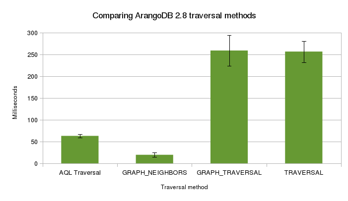
GRAPH_* functions and TRAVERSAL

ArangoDB also has a series of “Named Operations” that feature among
them a few that also do traversals. There is also a super old-school TRAVERSAL function hiding in the “Other” section. What’s interesting is how different their performance can be while still returning the same results.

I tested all of the traversal functions on the same supernode described above. These are the queries:

//AQL traversal
FOR v IN 2 ANY "vertices/1" edges
  FILTER v.name == "end"
    RETURN v

//GRAPH_NEIGHBORS
RETURN GRAPH_NEIGHBORS("db_10000", {_id: "vertices/1"}, {direction: "any", maxDepth:2, includeData: true, neighborExamples: [{name: "end"}]})

//GRAPH_TRAVERSAL
RETURN GRAPH_TRAVERSAL("db_10000", {_id:"vertices/1"}, "any", {maxDepth:2, includeData: true, filterVertices: [{name: "end"}], vertexFilterMethod: ["exclude"]})

//TRAVERSAL
RETURN TRAVERSAL(vertices, edges, {_id: "vertices/1"}, "any", {maxDepth:2, includeData: true, filterVertices: [{name: "end"}], vertexFilterMethod: ["exclude"]})

All of these returned the same vertex, just with varying levels of nesting within various arrays. Removing the nesting did not make a signficant difference in the execution time.

traversal_comparison
Traversing a supernode with 10000 incident edges with various traversal methods. N=5.

Notes

While TRAVERSAL and GRAPH_TRAVERSAL were not stellar performers here, the both have a lot to offer in terms of customizability. For ordering, depthfirst searches and custom expanders and visitors, this is the place to look. As you explore the options, I’m sure these get much faster.

Slightly less obvious but still worth pointing out that where AQL traversals require an id (“vertices/1000” or a document with and _id attribute), GRAPH_* functions just accept an example like {foo: “bar”} (I’ve passed in {_id: “vertices/1”} as the example just to keep things comparable). Being able to find things, without needing to know a specific id, or what collection to look in is very useful. It lets you abstract away document level concerns like collections and operate on a higher “graph” level so you can avoid hardcoding collections into your queries.

What it all means

The difference between these, at least superficially, similar traversals are pretty surprising. While some where faster than others, none of the options for tightening the scope of the traversal were used (edge restrictions, indexes, directionality). That tells you there is likely a lot of headroom for performance gains for all of the different methods.

The conceptual clarity that AQL traversals bring to the language as a whole is really nice, but it’s clear there is some optimization work to be done before I go and rewrite all my queries.

Where I have used the new AQL traversal syntax, I’m also going to have to check to make sure there are no unused v,e,p variables hiding in my queries. Where you need to use them, it looks like restricting yourself to v,e is the way to go. Generating those full paths is costly. If you use them, make sure it’s worth it.

Slowing Arango down is surprisingly instructive, but with 3.0 bringing the switch to Velocypack for JSON serialization, new indexes, and more, it looks like it’s going to get harder to do. :)


Data modeling with ArangoDB

Since 2009 there has been a “Cambrian Explosion” of NoSQL databases, but information on data modeling with these new data stores feels hard to come by.
My weapon of choice for over a year now has been ArangoDB. While ArangoDB is pretty conscientious about having good documentation, there has been something missing for me: criteria for making modeling decisions.

Like most (all?) graph databases, ArangoDB allows you to model your data with a property graph. The building blocks of a property graph are attributes, vertices and edges. What makes data modelling with ArangoDB (and any other graph database) difficult is deciding between them.

To start with we need a little terminology. Since a blog is a well known thing, we can use a post with some comments and some tags as our test data to illustrate the idea.

Sparse vs Compact

Modeling our blog post with as a “sparse” graph might look something like this:

sparse

At first glance it looks satisfyingly graphy: in the centre we see a green “Data Modeling” vertex which has a edge going to another vertex “post”, indicating that “Data Modeling” is a post. Commenters, tags and comments all have connections to a vertex representing their type as well.

Looking at the data you can see we are storing lots of edges and most vertices contain only a single attribute (apart from the internal attributes ArangoDB creates: _id, _key, _rev).

//vertices
{"_id":"vertices/26590247555","_key":"26590247555","_rev":"26590247555","title":"That's great honey","text":"Love you!"},
{"_id":"vertices/26590378627","_key":"26590378627","_rev":"26590378627","type":"comment"},
{"_id":"vertices/26590509699","_key":"26590509699","_rev":"26590509699","name":"Spammy McSpamerson","email":"spammer@fakeguccihandbags.com"},
{"_id":"vertices/26590640771","_key":"26590640771","_rev":"26590640771","title":"Brilliant","text":"Gucci handbags..."},
{"_id":"vertices/26590771843","_key":"26590771843","_rev":"26590771843","name":"arangodb"},
{"_id":"vertices/26590902915","_key":"26590902915","_rev":"26590902915","name":"modeling"},
{"_id":"vertices/26591033987","_key":"26591033987","_rev":"26591033987","name":"nosql"},
{"_id":"vertices/26591165059","_key":"26591165059","_rev":"26591165059","type":"tag"}]
 
//edges
[{"_id":"edges/26604010115","_key":"26604010115","_rev":"26604010115","_from":"vertices/26589723267","_to":"vertices/26589395587"},
{"_id":"edges/26607352451","_key":"26607352451","_rev":"26607352451","_from":"vertices/26589723267","_to":"vertices/26589854339"},
{"_id":"edges/26608204419","_key":"26608204419","_rev":"26608204419","_from":"vertices/26590640771","_to":"vertices/26590378627"},
{"_id":"edges/26609842819","_key":"26609842819","_rev":"26609842819","_from":"vertices/26590247555","_to":"vertices/26590378627"},
{"_id":"edges/26610694787","_key":"26610694787","_rev":"26610694787","_from":"vertices/26589985411","_to":"vertices/26590247555"},
{"_id":"edges/26611546755","_key":"26611546755","_rev":"26611546755","_from":"vertices/26589395587","_to":"vertices/26590247555"},
{"_id":"edges/26615020163","_key":"26615020163","_rev":"26615020163","_from":"vertices/26589985411","_to":"vertices/26590116483"},
{"_id":"edges/26618821251","_key":"26618821251","_rev":"26618821251","_from":"vertices/26590771843","_to":"vertices/26591165059"},
{"_id":"edges/26622622339","_key":"26622622339","_rev":"26622622339","_from":"vertices/26589395587","_to":"vertices/26589592195"},
{"_id":"edges/26625833603","_key":"26625833603","_rev":"26625833603","_from":"vertices/26590509699","_to":"vertices/26590640771"},
{"_id":"edges/26642741891","_key":"26642741891","_rev":"26642741891","_from":"vertices/26589395587","_to":"vertices/26590902915"},
{"_id":"edges/26645101187","_key":"26645101187","_rev":"26645101187","_from":"vertices/26589395587","_to":"vertices/26590771843"},
{"_id":"edges/26649885315","_key":"26649885315","_rev":"26649885315","_from":"vertices/26589395587","_to":"vertices/26591033987"},
{"_id":"edges/26651064963","_key":"26651064963","_rev":"26651064963","_from":"vertices/26590902915","_to":"vertices/26591165059"},
{"_id":"edges/26651785859","_key":"26651785859","_rev":"26651785859","_from":"vertices/26591033987","_to":"vertices/26591165059"},
{"_id":"edges/26652965507","_key":"26652965507","_rev":"26652965507","_from":"vertices/26590509699","_to":"vertices/26590116483"},
{"_id":"edges/26670267011","_key":"26670267011","_rev":"26670267011","_from":"vertices/26589395587","_to":"vertices/26590640771"}]

A “compact” graph on the other hand might look something like this:

{
  title: "Data modelling",
  text: "lorum ipsum...",
  author: "Mike Williamson",
  date: "2015-11-19",
  comments: [
    {
      author:"Mike's Mum",
      email:"mikes_mum@allthemums.com",
      text: "That's great honey",
    },
    {
      "author": "spammer@fakeguccihandbags.com",
      "title": "Brilliant",
      "text": "Gucci handbags...",
    }
  ],
  tags:["mongodb","modeling","nosql"]
}

Here we have taken exactly the same data and collapsed it together into a single document. While its a bit of a stretch to even classify this as a graph, ArangoDB’s multi-model nature largely erases the boundary between a document and a graph with a single vertex.

The two extremes above give us some tools for talking about our graph. Its the same data either way, but clearly different choices are being made. In the sparse graph, every vertex you see could have been an attribute, but was consciously moved into a vertex of its own. The compact graph is what comes out of repeated choosing to add new data as an attribute rather than a vertex.

When modeling real data your decisions don’t always fall one one side or the other. So what criteria should we be using to make those decisions?

Compact by default

As a baseline you should favor a compact graph. Generally data that is displayed together should be combined into a single document.

Defaulting to compact will mean fewer edges will exist in the graph as a whole. Since each traversal across a graph will have to find, evaluate and then traverse the edges for each vertex it encounters, keeping the number of edges to a strict minimum will ensure traversals stay fast as your graph grows.
Compact graphs will also mean fewer queries and traversals to get the information you need. When in doubt, embed. Resist the temptation to add vertices just because it’s a graph database, and keep it compact.

But not everything belongs together. Any attribute that contains a complex data structure (like the “comments” array or the “tags” array) deserves a little scrutiny as it might make sense as a vertex (or vertices) of its own.

Looking at our compact graph above, the array of comments, the array of tags, and maybe even the author might be better off as vertices rather than leaving them as attributes. How do we decide?

  • Will it be accessed on it’s own? (ie: showing comments without the post)
  • Will you be running a graph measurement (like GRAPH_BETWEENNESS) on it?
  • Will it be edited on it’s own?
  • Does/could the attribute have relationships of it’s own? (assuming you care)
  • Would/should this attribute exist without it’s parent vertex?

Removing duplicate data can also be a reason to make something a vertex, but with the cost of storage ridiculously low (and dropping) its a weak reason. Finding yourself updating duplicate data however, tells you that it should have been a vertex.

Edge Direction

Once you promote a piece of data to being a vertex (or “reify” it) your next decision is which way the edge connecting it to another vertex should go. Edge direction is a powerful way to put up boundaries to contain your traversals, but while the boundary is important the actual directions are not. Whatever you choose, it just needs to be consistent. One edge going the wrong direction is going to have your traversal returning things you don’t expect.

And another thing…

This post is the post I kept hoping to find as I worked on modeling my data with ArangoDB. Its not complete, data modeling is a big topic and there is lots more depth to ArangoDB to explore (ie: I haven’t yet tried splitting my edges amongst multiple edge collections) but these are some guidelines that I was hoping for when I was starting.

I would love to learn more about the criteria people are using to make those tough calls between attribute and vertex, and all those other hard modeling decisions.

If you have thoughts on this let me know!

ArangoDB’s geo-spatial functions

I’ve been playing with ArangoDB a lot lately. As a document database it looks to be a drop-in replacement for MongoDB, but it goes further, allowing graph traversals and geo-spatial queries.

Since I have a geo-referenced data set in mind I wanted to get to know its geo-spatial functions. I found the documentation a kind of unclear so I thought I would write up my exploration here.

At the moment there are only two geo-spatial functions in Arango; WITHIN and NEAR. Lets make some test data using the arango shell. Run arangosh and then the following:

db._create('cities')
db.cities.save({name: 'Ottawa', lat: 45.4215296, lng: -75.69719309999999})
db.cities.save({name: 'Montreal', lat: 45.5086699, lng: -73.55399249999999})
db.cities.save({name: 'São Paulo', lat: -23.5505199, lng: -46.63330939999999})

We will also need a geo-index for the functions to work. You can create one by passing in the name(s) of the fields that hold the latitude and longitude. In our case I just called them lat and lng so:

db.cities.ensureGeoIndex('lat', 'lng')

Alternately I could have done:

db.cities.save({name: 'Ottawa', location: [45.4215296, -75.69719309999999]})
db.cities.ensureGeoIndex('location')

As long as the values are of type double life is good. If you have some documents in the collection that don’t have the key(s) you specified for the index it will just ignore them.

First up is the WITHIN function. Its pretty much what you might expect, you give it a lat/lng and a radius and it gives you records with the area you specified. What is a little unexpected it that the radius is given in meters. So I am going to ask for the documents that are closest to the lat/lng of my favourite coffee shop (45.42890720357919, -75.68796873092651). To make the results more interesting I’ll ask for a 170000 meter radius (I know that Montreal is about 170 kilometers from Ottawa) so I should see those two cities in the result set:

arangosh [_system]> db._createStatement({query: 'FOR city in WITHIN(cities, 45.42890720357919, -75.68796873092651, 170000) RETURN city'}).execute().toArray()
[ 
  {
    "_id" : "cities/393503132620",
    "_rev" : "393503132620",
    "_key" : "393503132620",
    "lat" : 45.4215296,
    "lng" : -75.69719309999999,
    "name" : "Ottawa"
  },
  {
    "_id" : "cities/393504967628",
    "_rev" : "393504967628",
    "_key" : "393504967628",
    "lat" : 45.5086699,
    "lng" : -73.55399249999999,
    "name" : "Montreal"
  }
]

]

There is also an optional “distancename” parameter which, when given, prompts Arango to add the number of meters from your target point each document is. We can use that like this:

arangosh [_system]> db._createStatement({query: 'FOR city in WITHIN(cities, 45.42890720357919, -75.68796873092651, 170000, "distance_from_artissimo_cafe") RETURN city'}).execute().toArray()
[ 
  {
    "_id" : "cities/393503132620",
    "_rev" : "393503132620",
    "_key" : "393503132620",
    "distance_from_artissimo_cafe" : 1091.4226157106734,
    "lat" : 45.4215296,
    "lng" : -75.69719309999999,
    "name" : "Ottawa"
  },
  {
    "_id" : "cities/393504967628",
    "_rev" : "393504967628",
    "_key" : "393504967628",
    "distance_from_artissimo_cafe" : 166640.3086328647,
    "lat" : 45.5086699,
    "lng" : -73.55399249999999,
    "name" : "Montreal"
  } 
]

Arango’s NEAR function returns a set of documents ordered by their distance in meters from the lat/lng you provide. The number of documents in the set is controlled by the optional “limit” argument (which defaults to 100) and the same “distancename” as above. I am going to limit the result set to 3 (I only have 3 records in there anyway), and use my coffeeshop again:

arangosh [_system]> db._createStatement({query: 'FOR city in NEAR(cities, 45.42890720357919, -75.68796873092651, 3, "distance_from_artissimo_cafe") RETURN city'}).execute().toArray()
[ 
  {
    "_id" : "cities/393503132620",
    "_rev" : "393503132620",
    "_key" : "393503132620",
    "distance_from_artissimo_cafe" : 1091.4226157106734,
    "lat" : 45.4215296,
    "lng" : -75.69719309999999,
    "name" : "Ottawa"
  },
  {
    "_id" : "cities/393504967628",
    "_rev" : "393504967628",
    "_key" : "393504967628",
    "distance_from_artissimo_cafe" : 166640.3086328647,
    "lat" : 45.5086699,
    "lng" : -73.55399249999999,
    "name" : "Montreal"
  },
  {
    "_id" : "cities/393506343884",
    "_rev" : "393506343884",
    "_key" : "393506343884",
    "distance_from_artissimo_cafe" : 8214463.292795454,
    "lat" : -23.5505199,
    "lng" : -46.63330939999999,
    "name" : "São Paulo"
  } 
]

As you can see ArangoDB’s geo-spatial functionality is sparse but certainly enough to do some interesting things. Being able to act as a graph database AND do geo-spatial queries places Arango in a really interesting position and I am hoping to see its capabilities in both those areas expand. I’ve sent a feature request for WITHIN_BOUNDS, which I think would make working with leaflet.js or Google maps really nice, since it would save me doing a bunch of calculations with the map centre and the current zoom level to figure out a radius in meters for my query. I’ll keep my fingers crossed…

Update: My WITHIN_BOUNDS suggestion was actually implemented as WITHIN_RECTANGLE, and there is more geo stuff coming soon according to the roadmap.

Getting started with graph databases

I have a personal project I have been chipping away on for a little while now. I’ve been slowly adding more and more test data to it and as I do its become increasingly clear that while the data itself is neat, the stuff that is actually interesting is actually the relationships between the various entities and not so much the entities themselves. This realization led me to do some reading about graph databases. O’Reilly (as usual) has an interesting book on Graph Databases written by Ian Robinson, Jim Webber, and Emil Eifrem. Its a good intro but given that they hold positions of engineer, chief scientist and CEO at the company that makes the Neo4j graph database, its unsurprisingly focused on Neo4j.

Unfortunately the ‘j’ part of Neo4j refers to Java, which is a whole can of worms that I would rather not open. So I set off to look for a graph database that would not force me onto the JVM, or trap me with open-core licencing (or an $18,000 per year cost for my startup), and ultimately found ArangoDB.

Licenced under Apache 2, ArangoDB (formerly AvacadoDB) is a document database, in the same vein as MongoDB. What’s interesting is that it can also do key/value stuff like Redis and graphs like Neo4j.
Since its written in C++ I don’t have to worry about the JVM. So, lets get started with with it!

Installation is painless on Ubuntu:

wget -qO - http://www.arangodb.org/repositories/arangodb2/xUbuntu_13.10/Release.key | sudo apt-key add -
sudo sh -c "echo 'deb http://www.arangodb.org/repositories/arangodb2/xUbuntu_13.10/ /' > /etc/apt/sources.list.d/arangodb.list"
sudo apt-get update && sudo apt-get install arangodb

Since this is my first contact with graphs, I want a dataset that I can get a feel for working with graphs. Fortunately the company behind ArangoDB (triAGENS) has put some sample data up on github to get people started:

$> git clone https://github.com/triAGENS/ArangoDB-Data.git
Cloning into 'ArangoDB-Data'...
...
$> cd ArangoDB-Data/Graphs/IMDB
$> ./import.sh

That import script imports a bunch of IMDB data into ArangoDB and means that we can start exploring with the arango shell:

$> arangosh

                                       _     
  __ _ _ __ __ _ _ __   __ _  ___  ___| |__  
 / _` | '__/ _` | '_ \ / _` |/ _ \/ __| '_ \ 
| (_| | | | (_| | | | | (_| | (_) \__ \ | | |
 \__,_|_|  \__,_|_| |_|\__, |\___/|___/_| |_|
                       |___/                 

Welcome to arangosh 2.0.2 [linux]. Copyright (c) triAGENS GmbH
Using Google V8 3.16.14 JavaScript engine, READLINE 6.2, ICU 4.8.1.1

Pretty printing values.
Connected to ArangoDB 'tcp://localhost:8529' version: 2.0.2, database: '_system', username: 'root'

use 'help' to see common examples
arangosh [_system]>

Tab completion works super well here to give a sense of what your options are, but the first thing we care about is figuring out what that import did for us. You can see it created two collections (imdb_vertices and imdb_edges) with the db._collections() function:

arangosh [_system]> db._collections()
[ 
  [ArangoCollection 3021163, "_aal" (type document, status loaded)], 
  [ArangoCollection 1317227, "_graphs" (type document, status loaded)], 
  [ArangoCollection 3545451, "_replication" (type document, status loaded)], 
  [ArangoCollection 137579, "_users" (type document, status loaded)], 
  [ArangoCollection 1513835, "_cluster_kickstarter_plans" (type document, status loaded)], 
  [ArangoCollection 940644715, "vertices" (type document, status loaded)], 
  [ArangoCollection 3414379, "_aqlfunctions" (type document, status loaded)], 
  [ArangoCollection 1382763, "_modules" (type document, status loaded)], 
  [ArangoCollection 3610987, "_statistics" (type document, status loaded)], 
  [ArangoCollection 1160255851, "imdb_vertices" (type document, status loaded)], 
  [ArangoCollection 940710251, "edges" (type edge, status loaded)], 
  [ArangoCollection 3479915, "_trx" (type document, status loaded)], 
  [ArangoCollection 266194196843, "imdb_edges" (type edge, status loaded)], 
  [ArangoCollection 1448299, "_routing" (type document, status loaded)] 
]

We can also pick random documents out of the vertices collection with the .any() function to get a sense of whats in there.

 db.imdb_vertices.any()
{ 
  "_id" : "imdb_vertices/40233", 
  "_rev" : "6407199083", 
  "_key" : "40233", 
  "version" : 21, 
  "id" : "65952", 
  "type" : "Person", 
  "birthplace" : "", 
  "biography" : "", 
  "label" : "Jude Poyer", 
  "lastModified" : "1301901667000", 
  "name" : "Jude Poyer" 
}

If you have spent any time on the internet you will of course know that the obvious use for an IMDB graph is calculate Bacon numbers. So lets see if we can find Kevin in here:

arangosh [_system]> db._query('FOR Person IN imdb_vertices FILTER Person.name == "Kevin Bacon" RETURN Person').toArray()
[ 
  { 
    "_id" : "imdb_vertices/759", 
    "_rev" : "1218713963", 
    "_key" : "759", 
    "version" : 146, 
    "id" : "4724", 
    "type" : "Person", 
    "biography" : "", 
    "label" : "Kevin Bacon", 
    "lastModified" : "1299491319000", 
    "name" : "Kevin Bacon", 
    "birthplace" : "Philadelphia", 
    "profileImageUrl" : "http://cf1.imgobject.com/profiles/3e0/4bed49cf017a3c37a30003e0/kevin-bacon-profi...", 
    "birthday" : "-362451600000" 
  } 
]

And let’s see if we can connect him to, say, Kate Winslet. Since we know that Kevin is id imdb_vertices/759 and a little digging shows that Kate’s id is imdb_vertices/1088. We can pass those ids along with the imdb_vertices and imdb_edges collections to the SHORTEST_PATH function ArangoDB supplies for it to make the link between them:

arangosh [_system]> db._query('RETURN SHORTEST_PATH(imdb_vertices, imdb_edges, "imdb_vertices/759", "imdb_vertices/1088", "any", { maxIterations: 100000})').toArray()
[ 
  [ 
    { 
      "vertex" : { 
        "_id" : "imdb_vertices/759", 
        "_rev" : "1218713963", 
        "_key" : "759", 
        "version" : 146, 
        "id" : "4724", 
        "type" : "Person", 
        "biography" : "", 
        "label" : "Kevin Bacon", 
        "lastModified" : "1299491319000", 
        "name" : "Kevin Bacon", 
        "birthplace" : "Philadelphia", 
        "profileImageUrl" : "http://cf1.imgobject.com/profiles/3e0/4bed49cf017a3c37a30003e0/kevin-bacon-profi...", 
        "birthday" : "-362451600000" 
      } 
    }, 
    { 
      "vertex" : { 
        "_id" : "imdb_vertices/35451", 
        "_rev" : "5779626347", 
        "_key" : "35451", 
        "runtime" : 87, 
        "version" : 186, 
        "id" : "9692", 
        "genre" : "Drama", 
        "language" : "en", 
        "type" : "Movie", 
        "homepage" : "", 
        "tagline" : "", 
        "title" : "The Woodsman", 
        "label" : "The Woodsman", 
        "description" : "A pedophile returns to his hometown after 12 years in prison and attempts to sta...", 
        "imdbId" : "tt0361127", 
        "lastModified" : "1301903901000", 
        "imageUrl" : "http://cf1.imgobject.com/posters/3c1/4bc9281e017a3c57fe0103c1/the-woodsman-mid.j...", 
        "studio" : "Dash Films", 
        "releaseDate" : "1103842800000", 
        "released" : "2000-2010" 
      } 
    }, 
    { 
      "vertex" : { 
        "_id" : "imdb_vertices/1179", 
        "_rev" : "1274747243", 
        "_key" : "1179", 
        "version" : 90, 
        "id" : "335", 
        "type" : "Person", 
        "biography" : "", 
        "label" : "Michael Shannon", 
        "lastModified" : "1299902807000", 
        "name" : "Michael Shannon", 
        "profileImageUrl" : "http://cf1.imgobject.com/profiles/01c/4c2a3dc87b9aa15e9900001c/michael-shannon-p..." 
      } 
    }, 
    { 
      "vertex" : { 
        "_id" : "imdb_vertices/21077", 
        "_rev" : "3892517227", 
        "_key" : "21077", 
        "runtime" : 119, 
        "version" : 339, 
        "id" : "4148", 
        "genre" : "Drama", 
        "language" : "en", 
        "type" : "Movie", 
        "homepage" : "", 
        "tagline" : "", 
        "title" : "Revolutionary Road", 
        "label" : "Revolutionary Road", 
        "description" : "A young couple living in a Connecticut suburb during the mid-1950s struggle to c...", 
        "imdbId" : "tt0959337", 
        "trailer" : "http://www.youtube.com/watch?v=af01__Kvvr8", 
        "lastModified" : "1301907499000", 
        "imageUrl" : "http://cf1.imgobject.com/posters/627/4d4f8e275e73d617b7003627/revolutionary-road...", 
        "studio" : "BBC Films", 
        "releaseDate" : "1229641200000", 
        "released" : "2000-2010" 
      } 
    }, 
    { 
      "vertex" : { 
        "_id" : "imdb_vertices/1088", 
        "_rev" : "1262754155", 
        "_key" : "1088", 
        "version" : 102, 
        "id" : "204", 
        "type" : "Person", 
        "label" : "Kate Winslet", 
        "lastModified" : "1299746700000", 
        "name" : "Kate Winslet", 
        "birthplace" : "Reading, UK", 
        "profileImageUrl" : "http://cf1.imgobject.com/profiles/59f/4c022d0e017a3c702d00159f/kate-winslet-prof...", 
        "biography" : "<meta charset=\"utf-8\"><span style=\"font-family: sans-serif; font-size: 18px; lin...", 
        "birthday" : "181695600000" 
      } 
    } 
  ] 
]

So what we can see here is that it takes two hops (from Kevin to Michael Shannon via “The Woodsman“, and from Michael to Kate via “Revolutionary Road“), to connect Kevin Bacon to Kate Winslet, giving her a Bacon number of 2.

For the moment that is as far as I have gotten but I am pretty excited to explore the possiblities here. The more I think about graphs as a data model the more they seem to be a good fit for a lot of problems that I would normally be forcing into tables. Given that I can also just do straight document storage and the fact that they have a Object Document Mapper that works with Rails, I can tell you that ArangoDB and I will be spending a lot of time together.